An exploration of Graviton3 performance
Table of Contents
- 1. Introduction
- 2. Methodology
- 3. Target architectures and compilers
- 4. Experimental results
1. Introduction
This document presents an exploration of the performance of the Graviton3 processor using a set of carefully selected benchmarks.
The next sections cover the methodology as well as the benchmarking tool used to evaluate the performance of multiple CPU micro-architectures (Haswell, Skylake, Zen2 Rome, Zen3 Milan, and Graviton2) and compare their performance to the Graviton3.
2. Methodology
In order to evaluate the performance of the target systems, we deployed three categories of benchmarks that tackle different aspects:
1 - A CPU core frequency evaluation benchmark that uses a tight loop.
2 - A cache latency benchmark implementing a random pointer chasing loop aiming at measuring the latency of access to blocks of memory of different sizes.
3 - A set of code patterns representing common workloads found in production grade applications aiming at exposing the performance of the memory hierarchy of the target system. These benchmarks are also used to evaluate the quality of compiler generated code with regards to vectorization.
2.1. CPU core frequency benchmark
On AARCH64, the subs instruction is documented to require only 1 cycle to execute. This implies that we can implement a tight loop that can run in exactly N cycles (we assume the subs + bne is optimized and will cost only 1 cycle as well). Below is an example of such a loop for AARCH64:
__asm__ volatile (
                ".align 4\n"
                "loop1:\n"

                "subs %[_N], %[_N], #1\n"

                "bne loop1\n"

                : [_N] "+r" (N));
After timing this loop using clock_gettime for a given N, we can evaluate the frequency in GHz as follows: f = N / time in ns.
The same principle applies for x86_64, instead we used the following tight loop:
__asm__ volatile (
                "loop1:;\n"

                "dec %[_N];\n"

                "jnz loop1;\n"

                : [_N] "+r" (N));
2.2. Cache latency benchmark
This benchmark measures the latency of a memory access over a large array of pointers. The array is initialized using a random cyclic permutation that allows to access, for each iteration, a cacheline in a random order. This should break prefetching and expose the real access latency to a cache level.
Below are excerpts from the cyclic permutation code and the pointer chasing loop:
//Shuffle pointer addresses
for (int i = size - 1; i >= 0; i--)
  {
    if (i < cycle_len)
      continue;

    unsigned ii = yrand(i / cycle_len) * cycle_len + (i % cycle_len);

    void *tmp = memblock[i];

    memblock[i] = memblock[ii];
    memblock[ii] = tmp;
  }
p = &memblock[0];

for (int i = iterations; i; i--)
  {
    p = *(void **)p;
    p = *(void **)p;
    p = *(void **)p;
    p = *(void **)p;
    p = *(void **)p;
    p = *(void **)p;
    p = *(void **)p;
    p = *(void **)p;
    p = *(void **)p;
    p = *(void **)p;
    p = *(void **)p;
    p = *(void **)p;
    p = *(void **)p;
    p = *(void **)p;
    p = *(void **)p;
    p = *(void **)p;
  }
2.3. Memory bandwidth benchmarks
This section covers the C benchmarks and code patterns used to evaluate the bandwidth of the targeted systems.
The code patterns/workloads were inspired by the STREAM benchmark and mainly aim at exposing the system to various workloads mimicking the behavior of codelets commonly found in production applications.
Most of the chosen patterns should be 'easily' vectorized and parallelized (using OpenMP) by the available compilers.
In order to measure these benchmarks properly, many samples are collected and, for small array sizes, the kernels are repeated enough times to be accurately measurable. We also evaluate the stability/repeatability of the measurements by calculating the mean standard deviation of the collected samples and also evaluating the average error of the computations.
2.3.1. Load only benchmarks
These benchmarks perform only memory loads coupled with double precision floating-point arithmetic operations.
We will use the following symbols to express the global pattern of the benchmark: L for a load, S for a store, A for an addition, M for a multiplication, and F for FMA/MAC (Fused-Multiply-Add or Multiply-And-Accumulate) operations.
- Array reduction:

Figure 1: Array reduction formula
This code performs a load followed by an add. L,A pattern.
for (unsigned long long i = 0; i < n; i++)
  r += a[i];
- Dot product of two arrays:

Figure 2: Dotprod formula
This code performs two loads followed by a multiplication and addition operations. L,F pattern.
for (unsigned long long i = 0; i < n; i++)
  d += (a[i] * b[i]);
- Correlation factor between the data of two arrays:

Figure 3: Pearson correlation formula
The following code calculates the sums required to compute the correlation coefficient. L,L,A,F,A,F,F pattern.
for (unsigned long long i = 0; i < n; i++)
  {
    const double _a = a[i];
    const double _b = b[i];

    sum_a += _a;
    sum_a2 += (_a * _a);

    sum_b += _b;
    sum_b2 += (_b * _b);

    sum_ab += (_a * _b);
  }
- Least squares:

Figure 4: Least squares formula
This code calculates the sums required to compute the least square components m and b. L,L,A,F,A,F pattern.
for (unsigned long long i = 0; i < n; i++)
 {
   const double _a = a[i];
   const double _b = b[i];

   sum_a  += _a;
   sum_a2 += (_a * _a);

   sum_b  += _b;

   sum_ab += (_a * _b);
 }
2.3.2. Store and load/store benchmarks
These benchmarks perform load and store operations coupled with double precision floating-point arithmetic operations.
- Array initialization:

Figure 5: Array initialization formula
This code performs stores exclusively in order to initialize an array. S pattern.
for (unsigned long long i = 0; i < n; i++)
  a[i] = c;
- Array copy:

Figure 6: Array copy formula
This code performs a load and a store in order to copy an array into another. L,S pattern.
for (unsigned long long i = 0; i < n; i++)
  a[i] = b[i];
- Array scaling:

Figure 7: Array scaling formula
This code performs a load followed by a multiplication and a store. L,M,S pattern.
for (unsigned long long i = 0; i < n; i++)
  a[i] *= s;
- Array sum:

Figure 8: Array sum formula
This code performs two loads, an addition then a store. L,L,A,S pattern.
for (unsigned long long i = 0; i < n; i++)
  c[i] = (a[i] + b[i]);
- Triad:

Figure 9: Triad formula
This code performs three loads, a multiplication, an addition, then a store. L,L,F,S pattern.
for (unsigned long long i = 0; i < n; i++)
  c[i] += (a[i] * b[i]);
3. Target architectures and compilers
3.1. Target architectures
This table summarizes the main features of the targeted x86 and AARCH64 systems:
| Model name | Provider | Micro-architecture | Threads per core | Cores per socket | Sockets | Total cores | Total threads | Max freq. (GHz) | Boost freq. (GHz) | Min freq (GHz) | L1d (KiB) | L2 (KiB) | L3 (MiB) | L3/core (MiB) | SIMD ISA | Memory | Process |
|---|---|---|---|---|---|---|---|---|---|---|---|---|---|---|---|---|---|
| Intel(R) Xeon(R) E5-2699 v3 | LIPARAD | Haswell | 2 | 18 | 2 | 36 | 72 | 3.6 | False | 1.2 | 32 | 256 | 45 | 2.5 | SSE, AVX2 | DDR4 | 22 nm |
| Intel(R) Xeon(R) Platinum 8170 | LIPARAD | Skylake | 1 | 26 | 2 | 52 | 52 | 2.1 | False | 1.0 | 32 | 1024 | 35.75 | 1.375 | SSE, AVX2, AVX512 | DDR4 | 14 nm |
| Intel(R) Xeon(R) Platinum 8375C | AWS | Icelake | 2 | 24 | 1 | 24 | 48 | 3.5 | False | N/A | 48 | 512 | 54 | 2 | SSE, AVX2, AVX512 | DDR4 | 10 nm |
| AMD EPYC 7R32 | AWS | Zen2 Rome | 2 | 32 | 1 | 64 | 3.0 | 3.3 | N/A | 32 | 512 | 128 | 4 | SSE, AVX2 | DDR4 | 7 nm | |
| AMD EPYC 7R13 | AWS | Zen3 Milan | 2 | 32 | 1 | 64 | 3.0 | 3.7 | N/A | 32 | 512 | 128 | 4 | SSE, AVX2 | DDR4 | 7 nm | |
| Amazon Graviton2 | AWS | Neoverse N1 | 1 | 64 | 1 | 64 | 2.5 | False | N/A | 64 | 1024 | 32 | 0.5 | Neon | DDR4 | 7 nm | |
| Amazon Graviton3 | AWS | Neoverse V1 | 1 | 64 | 1 | 64 | 2.6 | False | N/A | 64 | 1024 | 32 | 0.5 | Neon, SVE | DDR5 | 5 nm |
3.2. Compilers available on x86 systems
3.2.1. Intel Haswell
- GCC version 11.2.0
- CLANG version 13.0.1
- Intel(R) oneAPI DPC++/C++ Compiler 2022.0.0 (2022.0.0.20211123)
- ICC 2021.5.0 20211109
3.2.2. Intel Skylake
- GCC version 11.2.0
- CLANG version 13.0.1
- Intel(R) oneAPI DPC++/C++ Compiler 2022.0.0 (2022.0.0.20211123)
- ICC 2021.5.0 20211109
3.2.3. Intel Ice Lake
- GCC version 11.x.x
- CLANG version 14.x.x
3.2.4. AMD Zen2 Rome
- GCC version 10.3.0
- AOCC version 3.2.0
3.2.5. AMD Zen3 Milan
- GCC version 10.3.0
- AOCC version 3.2.0
3.3. Compilers available on AARCH64 systems
3.3.1. Graviton2 (ARMv8.2 architecture/Neoverse N1 cores)
- GCC version 10.0.0
- CLANG version 12.0.0
- ARM 21.1
3.3.2. Graviton3 (ARMv8.4+SVE /Neoverse V1 cores)
- GCC version 11.1.0
- CLANG version 12.0.0
- ARM 21.1
4. Experimental results
4.1. Frequency benchmark
4.1.1. Single core
The following table shows the frequencies measured on a single core by running the frequency benchmark on the target systems:
| CPU model | Max Freq. in GHz | Measured freq. in GHz | Measurement error in % |
|---|---|---|---|
| Haswell | 3.6 | 3.5920 | 0.017 % |
| Skylake | 2.1 | 2.0904 | 0.015 % |
| Ice Lake | 3.5 | 3.5000 | 0.065 % |
| Zen2 Rome | 2.9 (3.3 with boost) | 3.3000 | 0.745 % |
| Zen3 Milan | 3.0 (3.7 with boost) | 3.7000 | 0.188 % |
| Graviton2 | 2.5 | 2.5000 | 0.037 % |
| Graviton3 | 2.6 | 2.6000 | 0.008 % |
From the measurements above, we can safely conclude that the systems are quite stable and that performance measurements won't be affected by CPU frequency fluctuations due to DVFS, Frequency Boost, or some other power/frequency management technology.
4.1.2. Multi-core
The following plots show the measured frequency across multiple cores in parallel. The benchmark is run on 1, 2, 3, 4, … cores at a time and the measured frequency for each core is recorded along with the measurement stability.
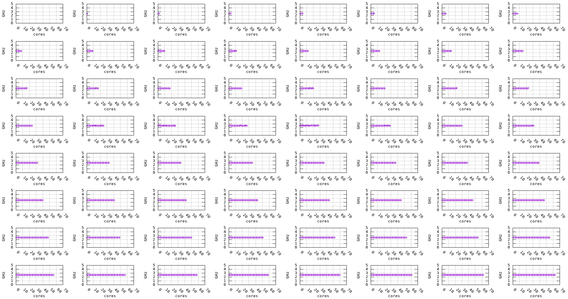
Figure 10: Graviton2 frequency evolution accross multiple cores (2.5GHz)
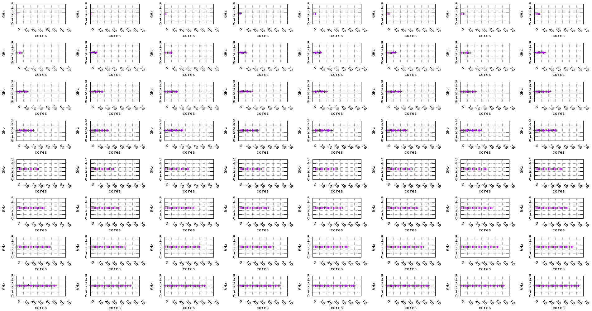
Figure 11: Graviton3 frequency evolution accross multiple cores (2.6GHz)
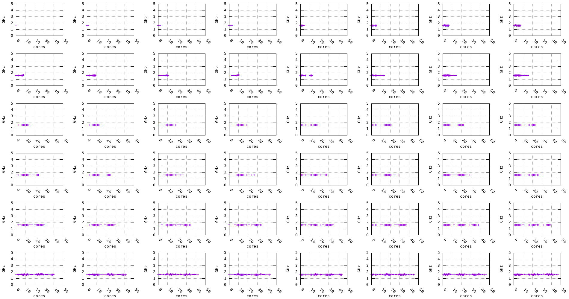
Figure 12: A64FX frequency evolution accross multiple cores (2.6GHz)
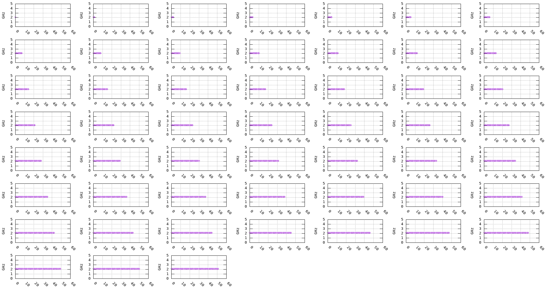
Figure 13: Skylake frequency evolution accross multiple cores (2.1GHz)
We can notice for the Graviton2, Graviton3, and Skylake processors that, regardless of the number of cores being used, the frequency remains stable. On the other hand, for the Zen2, Zen3, and Haswell processors, the frequency seems to drop when multiple cores are being used, as shown in the plots below.
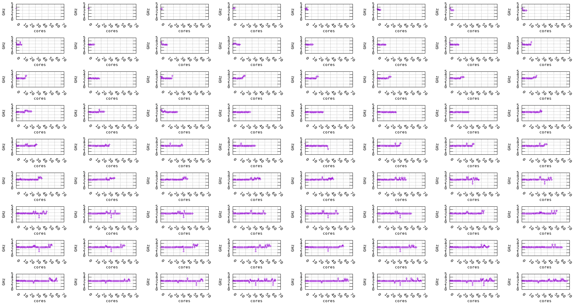
Figure 14: Haswell frequency evolution accross multiple cores
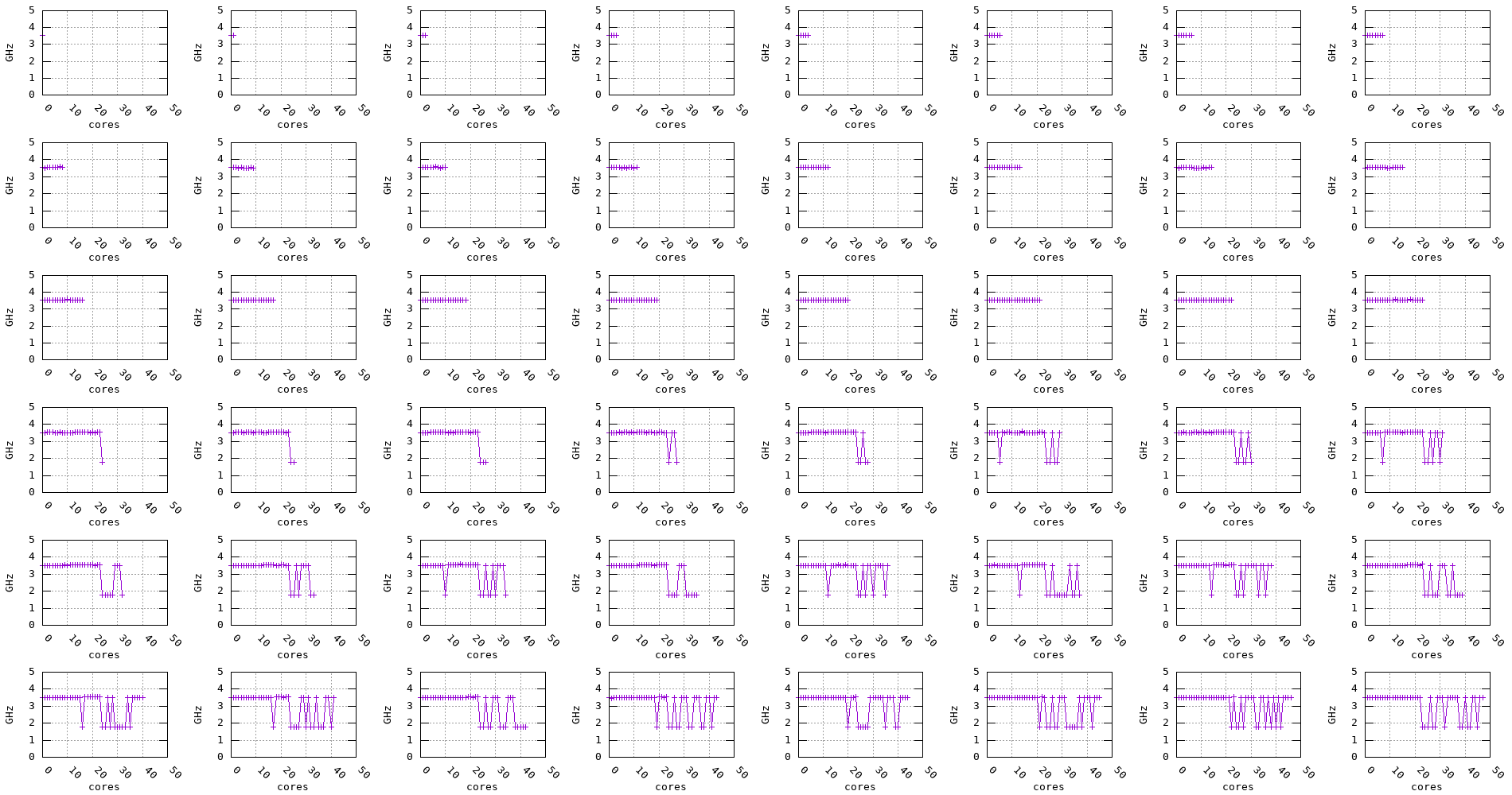
Figure 15: Icelake frequency evolution accross multiple cores
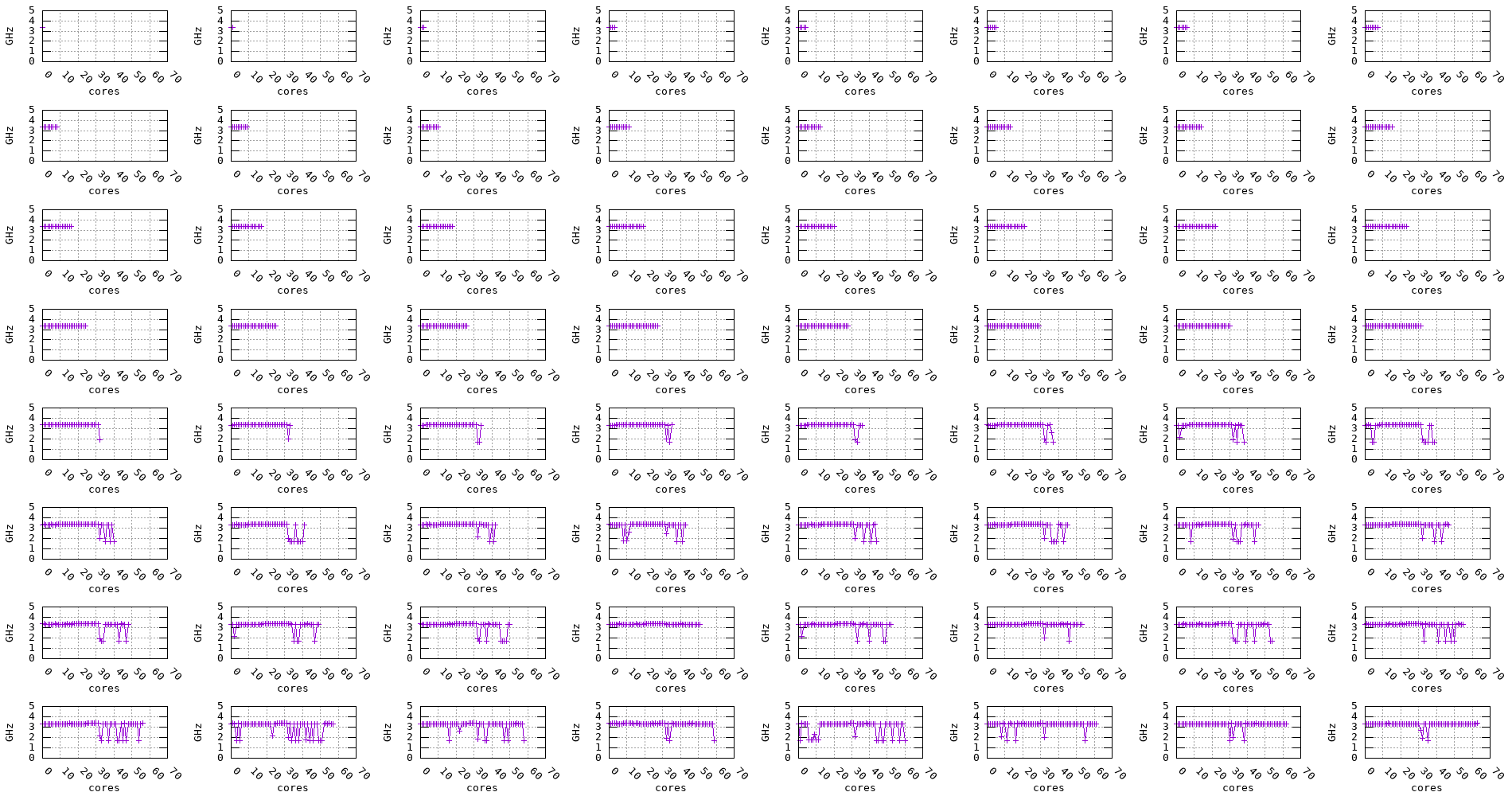
Figure 16: Zen2 frequency evolution accross multiple cores
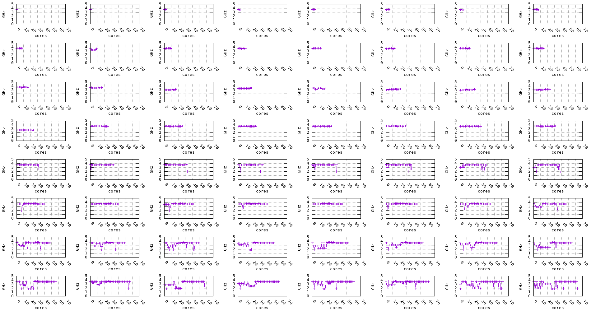
Figure 17: Zen3 frequency evolution accross multiple cores
4.2. Cache benchmark
The following figures show the results of the cache benchmark (random pointer chasing) on the architectures described above.
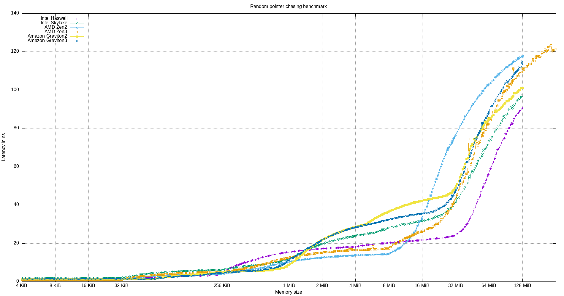
Figure 18: Cache latency benchmark on multiple CPU micro-architectures
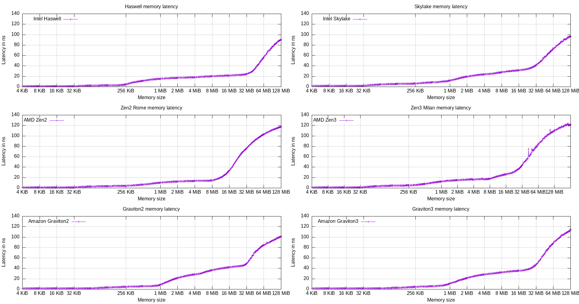
Figure 19: Cache latency benchmark on multiple CPU micro-architectures (split)
Here, we compare the cache latency of the Graviton3 CPU to the other CPUs.
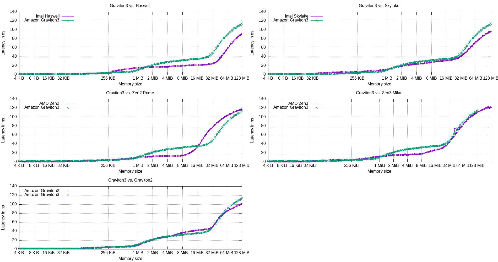
Figure 20: One-to-one comparison of the cache latencies of Graviton3 and other CPU micro-architectures
4.3. Bandwidth benchmarks
4.3.1. Single core benchmarks
The following tables summarize the bandwidth (in GiB/s) for each benchmark on the target systems using multiple compilers.
Important: Note that the results shown here do not necessartily reflect the best performance of the underlying architecture, rather, the performance of compiler generated code.
- GCC
- -O3 -funroll-loops -finline-functions
Model name init copy scale sum triad reduc dotprod correl leatssq Haswell 7.841 20.752 8.126 11.036 11.274 7.082 10.960 7.855 8.974 Skylake 8.788 9.331 10.911 11.400 11.384 3.817 7.365 6.382 6.658 Ice Lake 11.260 30.527 13.400 14.075 13.856 6.102 11.418 9.990 10.294 AMD EPYC Zen2 Rome 14.571 18.046 16.267 22.972 25.646 7.647 14.656 12.599 13.336 AMD EPYC Zen3 Milan 18.644 36.567 23.008 24.410 28.370 8.702 17.343 12.408 16.254 Amazon Graviton2 36.929 30.881 16.889 24.456 14.988 9.062 17.634 11.748 13.778 Amazon Graviton3 49.597 49.897 25.261 45.530 33.536 9.637 19.270 11.015 13.931 A64FX 23.587 15.173 23.350 42.082 37.020 1.473 2.912 4.360 12.567 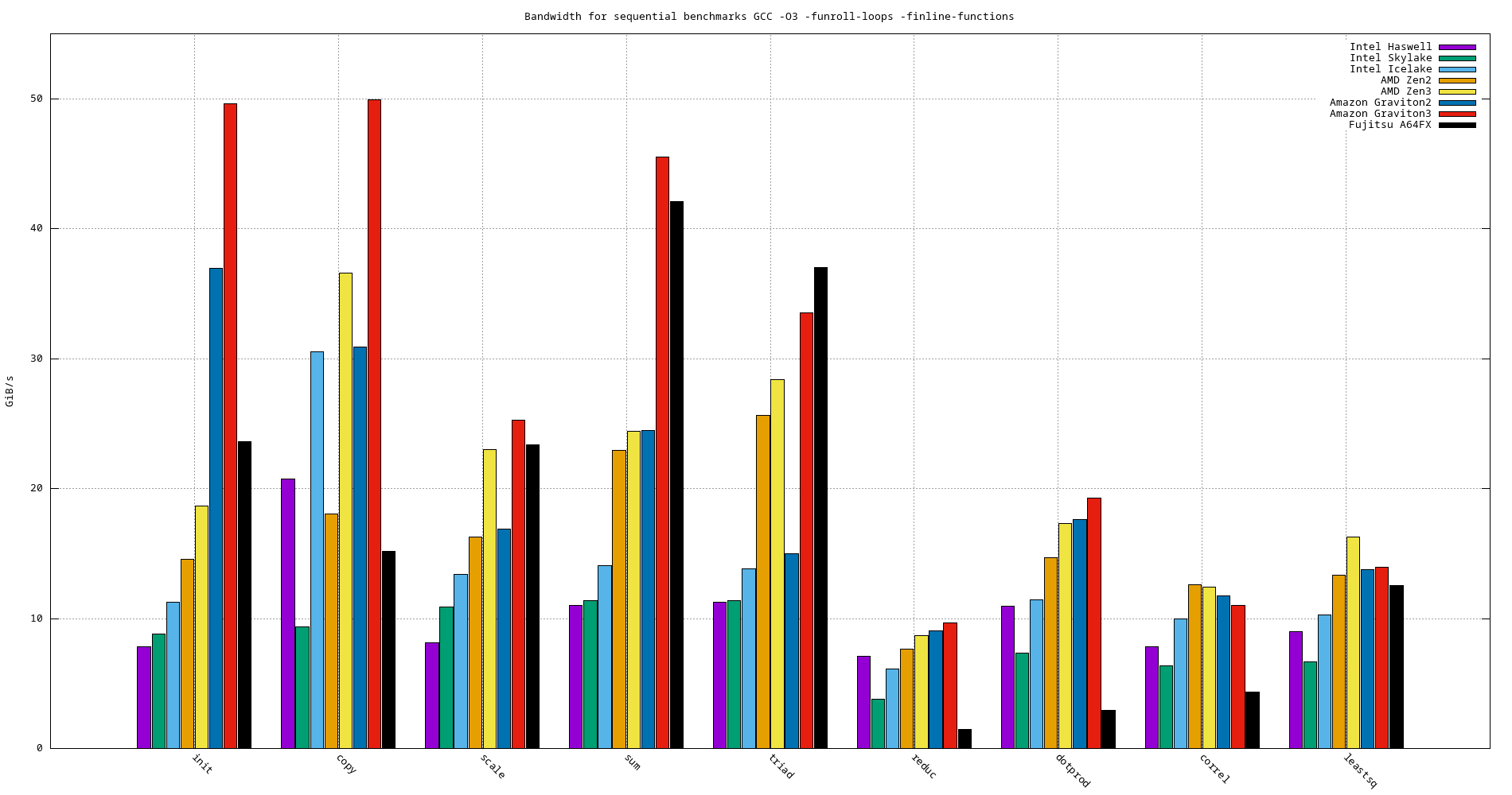
Figure 21: Bandwidth benchmarks
- -Ofast -funroll-loops -finline-functions
Model name init copy scale sum triad reduc dotprod correl leatssq Haswell 7.974 20.882 8.169 8.169 11.097 11.349 12.408 11.790 11.909 Skylake 8.579 9.293 10.780 11.332 11.332 11.152 11.777 10.898 11.083 Ice Lake 11.156 29.792 13.264 14.042 13.823 14.185 13.853 14.689 14.105 AMD EPYC Zen2 Rome 14.321 18.103 16.066 23.109 25.740 17.181 23.563 22.084 22.829 AMD EPYC Zen3 Milan 18.045 34.784 22.307 24.938 28.810 25.937 31.717 30.118 30.519 Amazon Graviton2 36.814 31.698 18.646 24.044 17.396 17.427 18.386 18.620 18.618 Amazon Graviton3 49.654 49.971 24.965 45.835 33.573 28.084 34.672 34.077 34.348 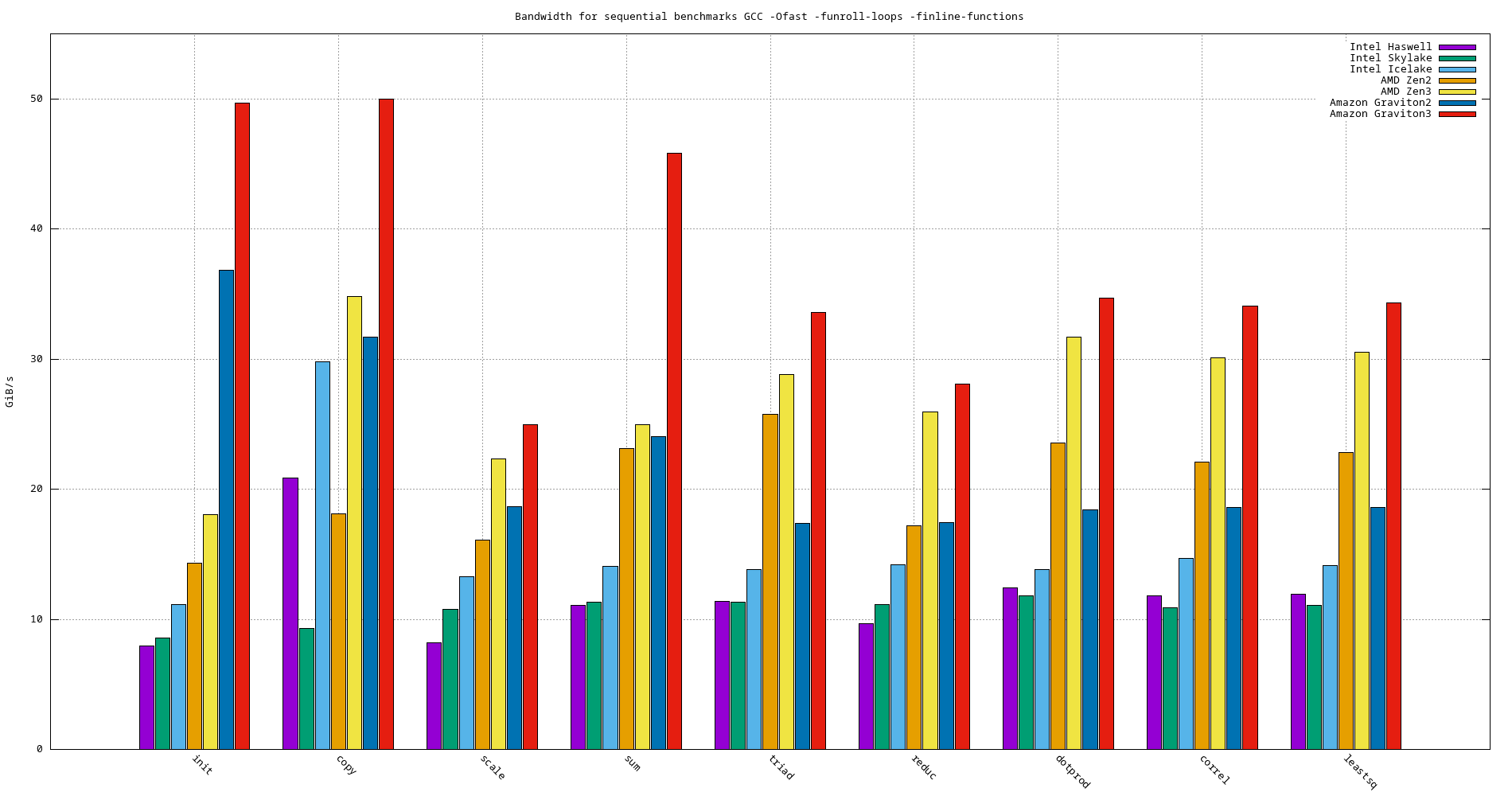
Figure 22: Bandwidth benchmarks
- -O3 -funroll-loops -finline-functions
4.3.2. Parallel benchmarks (OpenMP)
The following table summerizes the performance (in GiB/s) for all parallel benchmarks on the target systems using multiple compilers:
- GCC
- -O3 -fopenmp -funroll-loops -finline-functions
Model name init copy scale sum triad reduc dotprod correl leastsq Haswell 40.472 59.449 40.031 67.926 67.875 97.832 96.924 96.812 96.819 Skylake 85.154 113.010 55.220 107.421 128.508 126.979 166.585 174.954 172.813 Ice Lake 70.676 121.012 60.045 128.628 103.566 139.729 145.405 143.077 143.379 AMD EPYC Zen2 Rome 39.121 56.896 47.520 72.865 75.696 73.042 92.864 92.334 92.486 AMD EPYC Zen3 Milan 57.402 78.408 59.934 87.267 87.069 111.427 116.127 115.192 114.831 Amazon Graviton2 148.458 146.693 74.474 149.744 111.612 146.820 153.409 152.044 151.884 Amazon Graviton3 213.623 232.102 110.914 223.261 182.721 251.491 260.696 260.398 260.879 A64FX 364.709 460.137 378.337 446.239 483.873 70.101 137.800 65.379 82.239 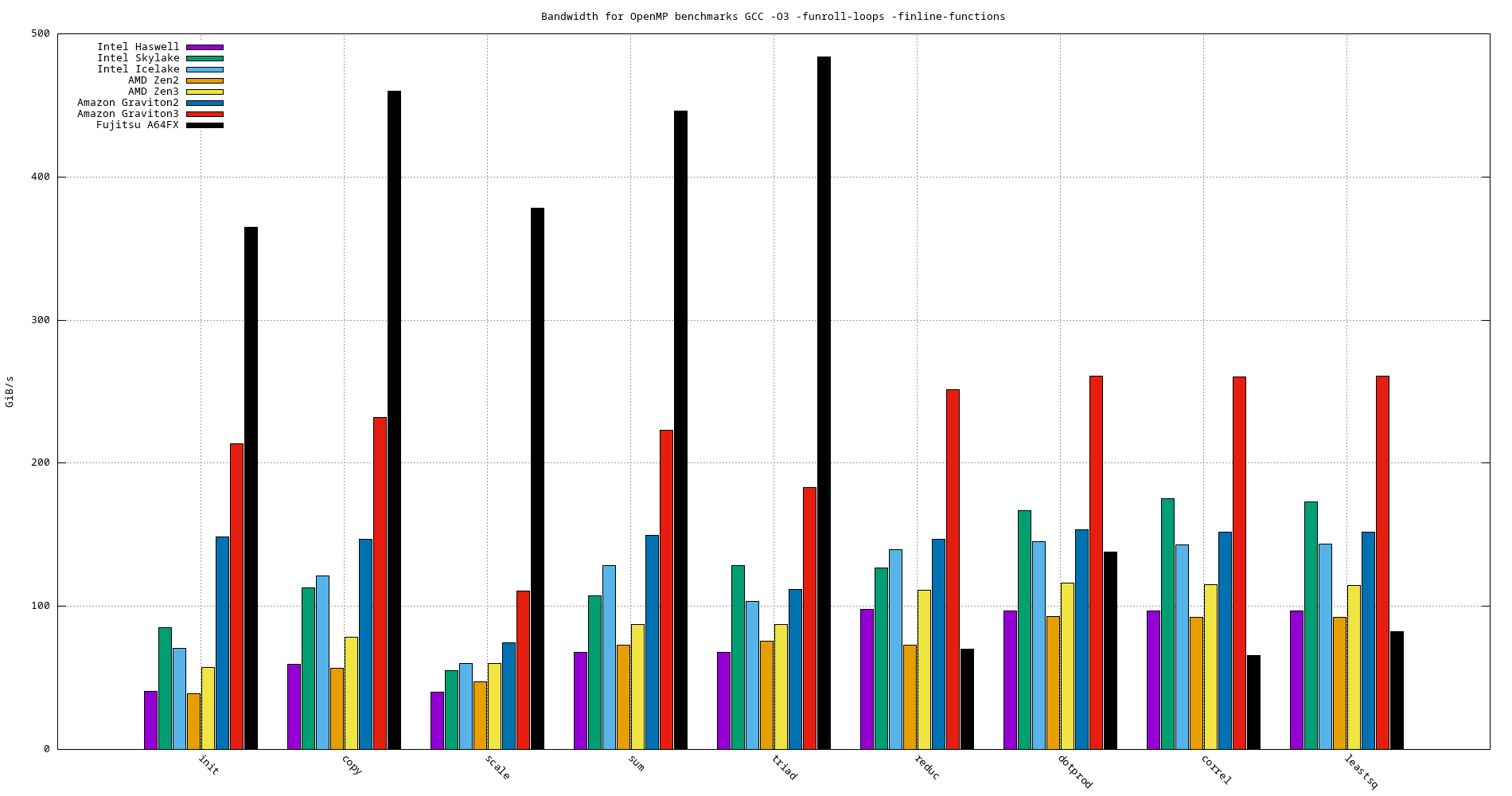
Figure 23: Bandwidth benchmarks
- -Ofast -fopenmp -funroll-loops -finline-functions
Model name init copy scale sum triad reduc dotprod correl leastsq Haswell 40.145 60.237 40.187 67.652 67.642 98.684 94.644 96.378 94.922 Skylake 83.874 110.347 86.372 126.957 126.106 193.222 168.237 176.408 175.184 Ice Lake 70.808 121.963 60.427 128.920 103.579 145.062 147.960 146.683 146.861 AMD EPYC Zen2 Rome 47.723 65.030 48.859 75.014 75.361 80.624 91.055 87.829 93.232 AMD EPYC Zen3 Milan 57.140 78.207 59.888 87.296 87.416 112.586 115.968 116.036 115.920 Amazon Graviton2 145.616 145.986 74.299 149.841 111.622 147.861 153.018 151.939 151.882 Amazon Graviton3 216.010 232.508 110.993 223.247 183.110 258.779 259.508 260.373 260.067 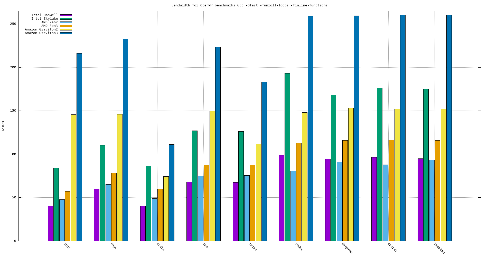
Figure 24: Sequential bandwidth benchmarks comparison
- -O3 -fopenmp -funroll-loops -finline-functions
- Sequential side-by-side comparison
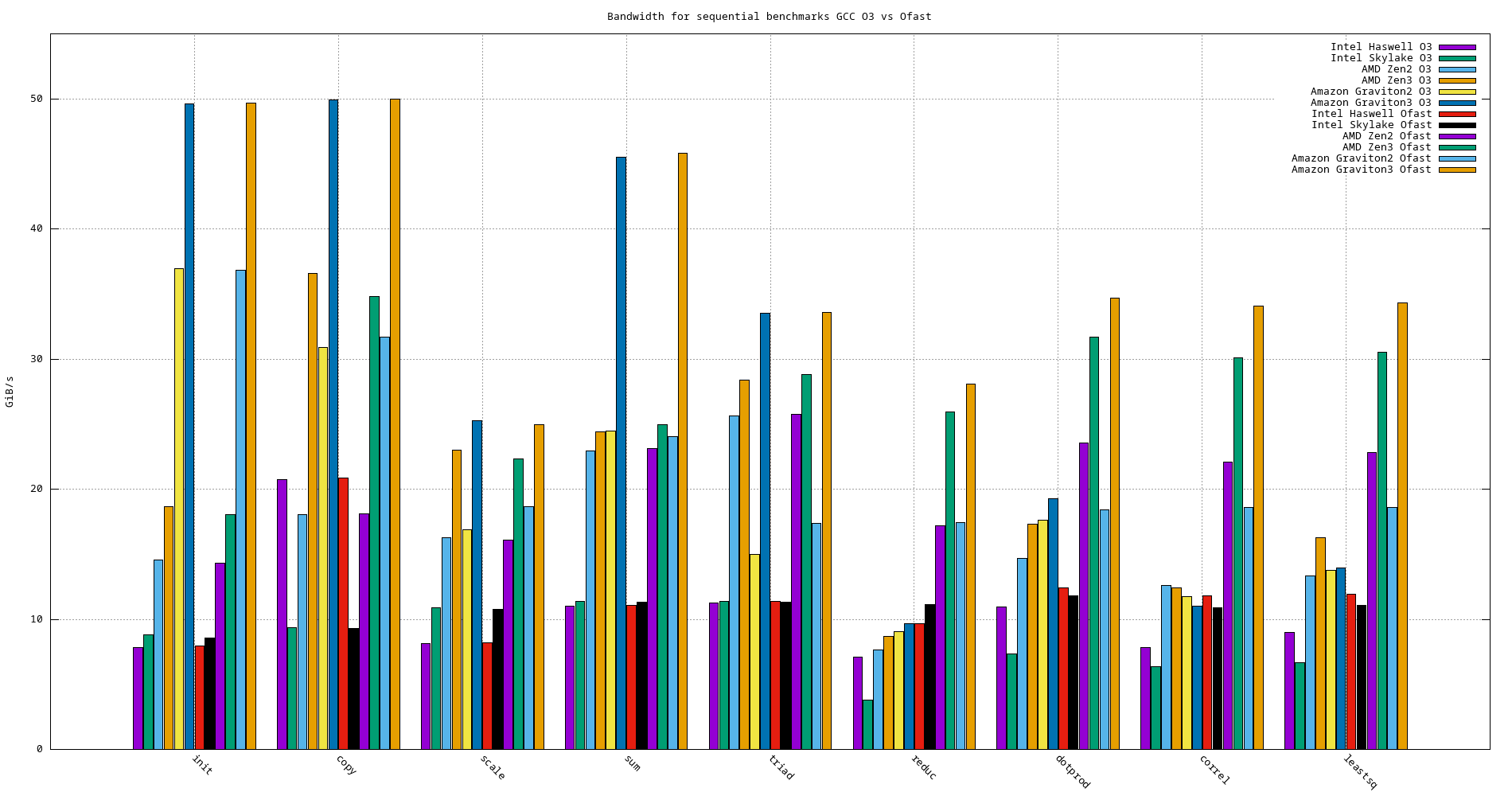
Figure 25: OpenMP bandwidth benchmarks comparison
4.4. Graviton3 compilers comparison
4.4.1. GCC
- assembly codes (soon …)
4.4.2. CLANG
- assembly codes (soon …)
4.4.3. ARM CLANG
- assembly codes (soon …)
4.4.4. Sequential benchmarks
| Compiler | init | copy | scale | sum | triad | reduc | dotprod | correl | leastsq |
|---|---|---|---|---|---|---|---|---|---|
| GCC | 49.597 | 49.897 | 25.261 | 45.530 | 33.536 | 9.637 | 19.270 | 11.015 | 13.931 |
| CLANG | 57.860 | 49.673 | 25.126 | 45.665 | 33.334 | 9.630 | 19.106 | 13.08 | 16.034 |
| ARM CLANG | 57.171 | 49.698 | 25.084 | 45.649 | 33.357 | 9.631 | 19.090 | 13.101 | 15.959 |
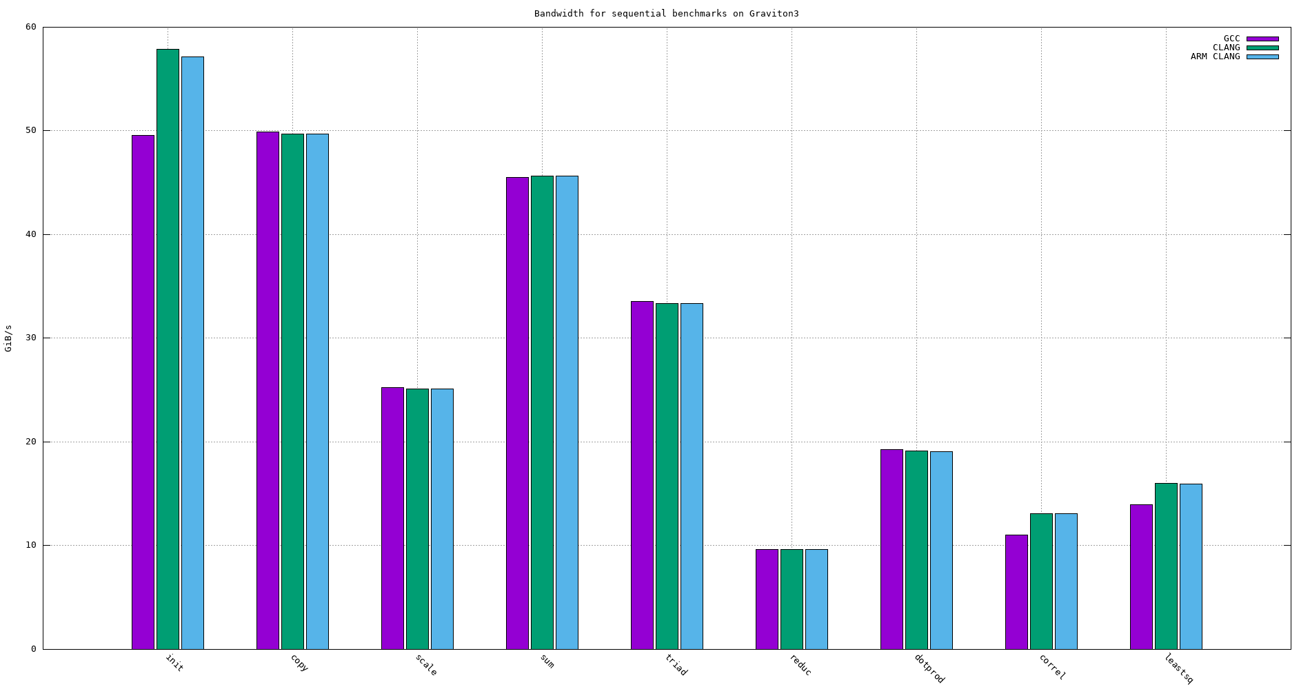
Figure 26: Sequential bandwidth of the different compilers on Graviton3 -O3 -funroll-loops -finline-functions
4.4.5. OpenMP benchmarks
| Compiler | init | copy | scale | sum | triad | reduc | dotprod | correl | leastsq |
|---|---|---|---|---|---|---|---|---|---|
| GCC | 213.623 | 232.102 | 110.914 | 223.261 | 182.721 | 251.491 | 260.696 | 260.398 | 260.879 |
| CLANG | 218.906 | 232.225 | 111.093 | 221.840 | 183.534 | 251.695 | 260.299 | 258.103 | 259.629 |
| ARM CLANG | 217.381 | 231.842 | 110.995 | 222.039 | 183.397 | 251.372 | 260.351 | 257.790 | 259.489 |
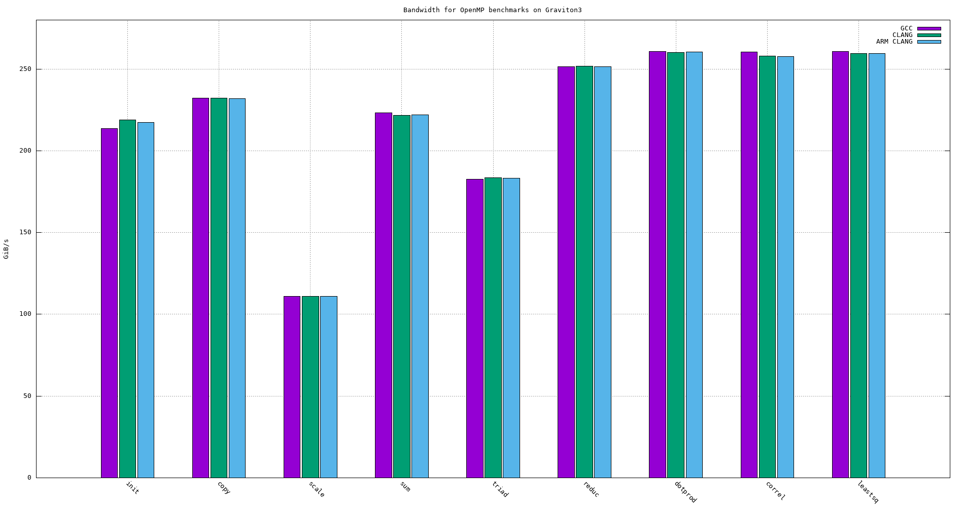
Figure 27: OpenMP bandwidth for different compilers on Graviton3 -O3 -funroll-loops -finline-functions
4.5. A64FX
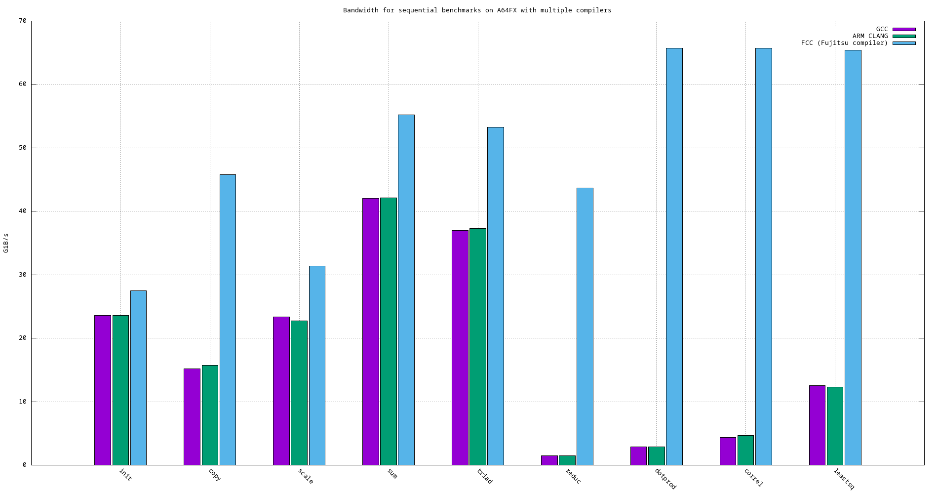
Figure 28: Bandwidth of sequential benchmarks using different compilers on A64FX
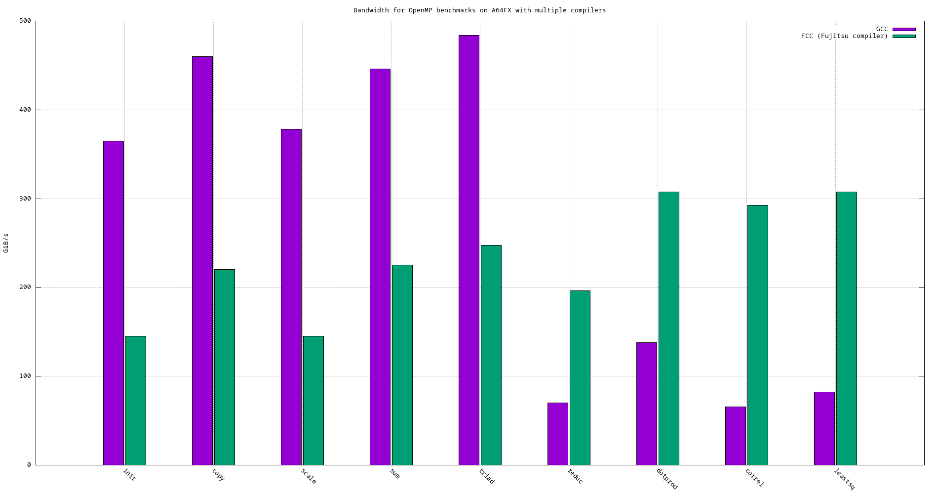
Figure 29: Bandwidth of OpenMP benchmakrs using different compilers on A64FX
4.6. Graviton3 vs. A64FX
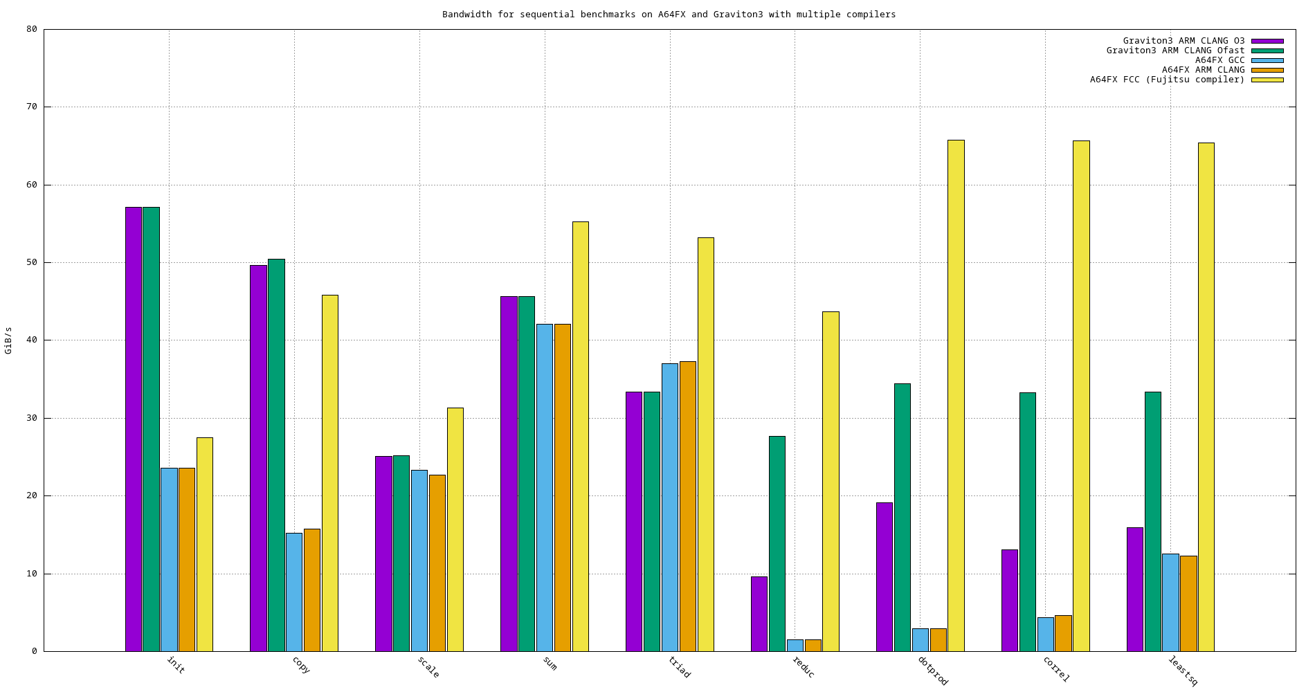
Figure 30: Bandwidth comparison of sequential benchmarks using different compilers on A64FX and Graviton3
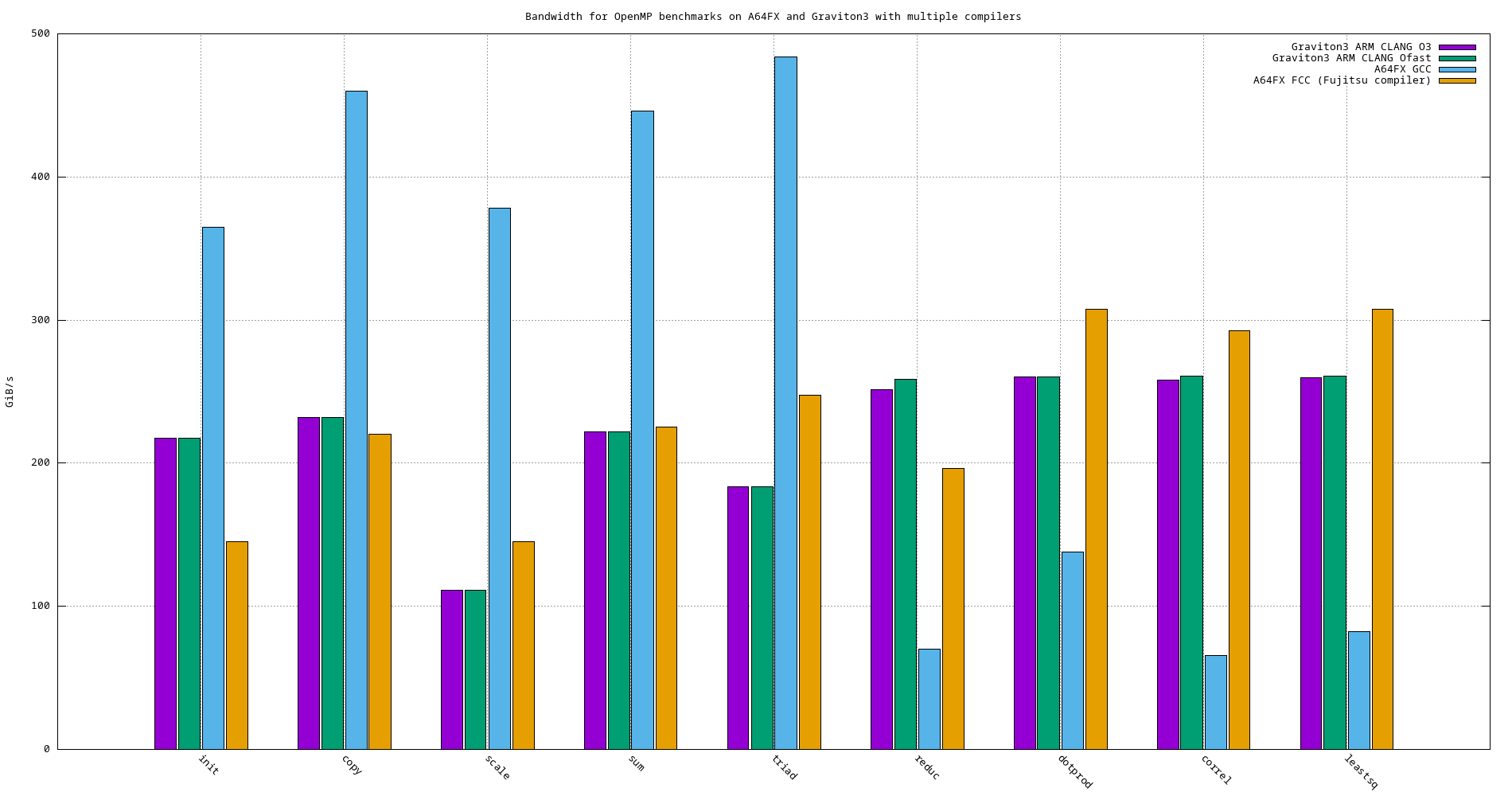
Figure 31: Bandwidth comparison of OpenMP benchmarks using different compilers on A64FX and Graviton3